Cool stuff: Lab 01

In this cool stuff, I just have a few things to share including, commenting in Quarto and R, literature search 2.0, bibliographies, citation and reference styles, Quarto + other languages, and a first look at figures.

As always, I hope you find this information helpful and interesting!

Using commenting in Quarto and R

When writing documents in Quarto, you will often find yourself in a situation in which you would like to write some comments in the prose that only you will see and that will not appear in the final document. Think of these comments as notes to yourself (or to your collaborators). It’s like ‘speaker notes’ for slide presentations.

In Markdown, you can use HTML comments to achieve this. For example, the following HTML comment will not appear in the final document:

## This is a heading

<!-- This is a comment that will not appear in the final document -->

Here is my prose....

In your labs, project steps, and self-assessments these comments may be helpful to you as you work through the steps and document the questions you need to answer or ideas that you have that will help you complete the task.

When we write in code block, the comments have a different purpose. They are used to explain the code to others (and to yourself in the future). The comments will appear (if you use the echo: true option) in the final document. Here is an example of a comment in R:

# Print my name
print("My name is Jerid Francom")

I hope that these comments will help you as you work through the labs and projects!

Literature search 2.0

The WFU ZSR Library provides access for the WFU community to a couple of research tools that can help you with your literature search. These tools use AI to help you find the most relevant articles for your research. They are called Elicit and Scite.

(a)

(b)

Figure 1: AI tools for literature search

Create an account with your WFU email and start using these tools to find the most relevant articles for your research!

Bibliographies

In the previous lab, we learned how to add citations to our documents. By first adding the bibliography: key to the YAML front matter with a *.bib file as the value and then adding the @ symbol followed by the citation key in the prose.

The somewhat more tricky aspect is getting the reference entries in the BiBTeX format. Once you have identified a source that you want to cite, you can sometimes find a link to create a BibTeX entry –but many times not.

In the latter case, you can use a DOI (Digital Object Identifier) and the doi2bib.org website to create the BiBTeX entry. Just identify the DOI, which generally appears in the article’s metadata and has the form 10.1234/5678 (or something similar) and paste it into the website. The website will generate the BiBTeX entry for you. You can copy and paste this entry into your *.bib file. Use the citation key in the @ symbol in the prose of your Quarto document.

Citation and reference styles

The BibTeX format is only a storage format. The style of the citations and the bibliography is determined by the style file that you use. The default style file in Quarto is the Chicago Manual of Style.

You can change the style file by downloading a new style file (.csl), adding it to your project, and then using the csl: key in the front matter to specify the new style file.

Figure 2: Adding a new .csl file to your project

Quarto + other languages

Quarto is a great tool for writing documents in which we combine prose (in Markdown) and R. But you should know that Quarto can also be used with other languages, such as Python, Julia, and Observable JavaScript. This is a great feature, as it allows you to use the best tool for the job, and to combine different languages in the same document!

Listing 1: R code

x <- c(1, 2, 3)
y <- c(4, 5, 6)

x %*% y

     [,1]
[1,]   32

Listing 2: Python code

import numpy as np

x = np.array([1, 2, 3])
y = np.array([4, 5, 6])

np.dot(x, y)

32

At the moment you have enough on your hands with Quarto + R. But it’s good to know that you can expand your horizons in the future!

First look: figures

I know a lot of you are really excited to get to the point where you can add figures to your documents. We cover figures head on soon!

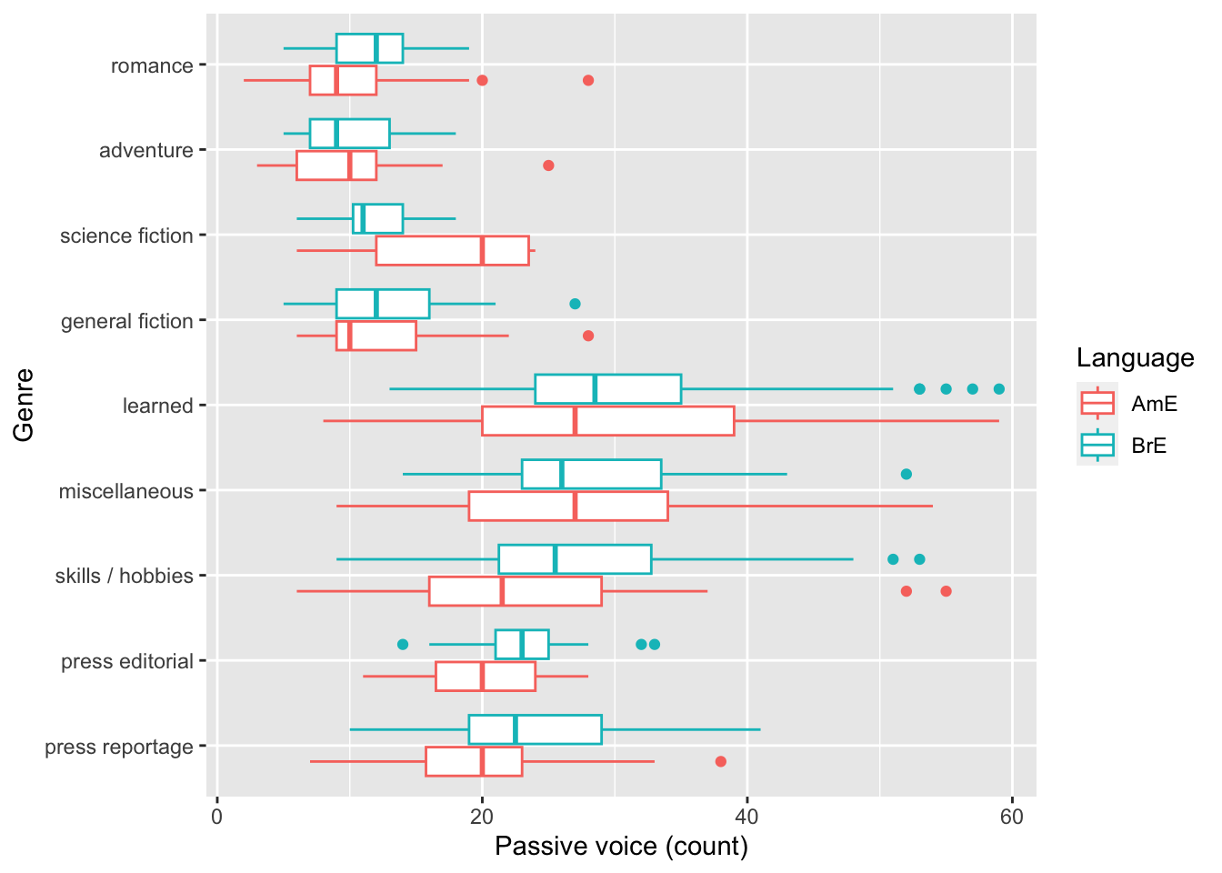
For now, I want to introduce you to the ggplot2 package, which is a great tool for creating figures in R. In Figure 3 I don’t expect you to understand this code, but if you are interested and have some time, you can take a look at the code and see if you can understand what it does.

```{r}
#| label: fig-brown-lob
#| fig-cap: "Passive voice in the Brown (AmE) and LOB (BrE) corpora"

# Load packages
library(ggplot2)      # for plotting
library(dplyr)        # for data manipulation
library(corpora)      # for the BrownLOBPassives dataset

# Get the dataset
data <- BrownLOBPassives |> as_tibble()

# Create boxplot
data |>
  ggplot(aes(
    x = genre,
    y = passive,
    color = lang
    )) +
  geom_boxplot() +
  labs(
       x = "Genre",
       y = "Passive voice (count)",
       color = "Language"
       ) +
    coord_flip()
```

Figure 3: Passive voice in the Brown (AmE) and LOB (BrE) corpora